Wonder Woman | Captain Marvel |
---|---|
![]() |
![]() |
Women are involved in the film industry in all roles, including as film directors, actresses, cinematographers, film producers, film critics, and other film industry professions, though women have been underrepresented in all these positions. Studies found that women have always had a presence in film acting, but have consistently been underrepresented, and on average significantly less well paid.
In 2015, Forbes reported that "...just 21 of the 100 top-grossing films of 2014 featured a female lead or co-lead, while only 28.1% of characters in 100 top-grossing films were female... This means it’s much rarer for women to get the sort of blockbuster role which would warrant the massive backend deals many male counterparts demand (Tom Cruise in Mission: Impossible or Robert Downey Jr. in Iron Man, for example)".
Also, Forbes' analysis of US acting salaries in 2013 determined that the "...men on Forbes’ list of top-paid actors for that year made 2½ times as much money as the top-paid actresses. That means that Hollywood's best-compensated actresses made just 40 cents for every dollar that the best-compensated men made.
We will look to examine whether and how women representation is lacking in the film industry. To do this, we will adopt The Bechdel test as a measure of the representation of women in the film industry. The test is named after the American cartoonist Alison Bechdel in whose 1985 comic strip Dykes to Watch Out For the test first appeared.
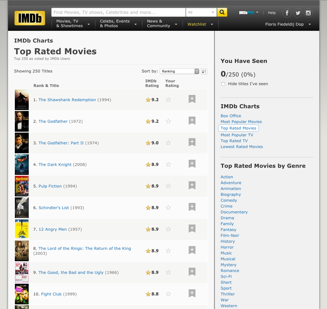
We will get the data ourselves to perform the analysis. Specifically, we will retrieve the movie metadata from IMDB (Internet Movie Database), an online database of information related to films, television programs, home videos, video games, and streaming content online – including cast, production crew and personal biographies, plot summaries, trivia, ratings, and fan and critical reviews. As of January 2021, IMDb has approximately 6.5 million titles (including episodes) and 10.4 million personalities in its database, as well as 83 million registered users.
The IMDb Top 250 is a list of the top rated 250 films, based on ratings by the registered users of the website using the methods described. We will focus on these famous movies in this analysis:
We will retrieve the metadata of IMDb Top 250 movies from the IMDb charts. For each movie on the list, we can scrape the following characteristics from the information page. For example, from the page of top rated movie "The Shawshank Redemption", we want to extract the metadata about this movie as:
import pandas as pd
import numpy as np
import requests
from bs4 import BeautifulSoup
# Question 1.1
page = requests.get("https://www.imdb.com/chart/top/")
page
soup = BeautifulSoup(page.content, 'html.parser')
# We have found that the first title starts at line 59 of the code
tag = soup.find_all("a")[60]
link = tag['href']
link
link_dic = {}
rank = 0
# We add a step in the range since the links appear twince for the same title (image and url) and both go to the same place
for row in range(60, len(soup.find_all("a"))-54, 2):
rank += 1
temporary = soup.find_all("a")[row]
link_dic[rank] = temporary['href']
data = {}
rank = []
imdb_id = []
title = []
year = []
director = []
starring = []
rating = []
n_reviews = []
genre = []
country = []
box_off_rev = []
language = []
budget = []
runtime = []
for i in range(1,250+1):
# Link to be scrapped
half_url = link_dic[i]
headers = {'Accept-Language': 'en-US, en;q=0.5'}
page = requests.get("https://www.imdb.com/"+half_url, headers = headers)
new_soup = BeautifulSoup(page.content, 'html.parser')
# Rank
rank.append(i)
data['Rank'] = rank
# IMDBid
imdb_id.append(str(half_url[9:-1]))
data['imdb_id'] = imdb_id
# Movie Name
t = new_soup.find(class_='title_wrapper').get_text().strip()
tit = ''
for i in t:
if i == '\xa0':
break
tit+=i
title.append(tit)
data['Movie'] = title
# Find the Year
y = new_soup.find(attrs = {'id':'titleYear'}).get_text()
year_1 = [i for i in y if i not in ['(',')']]
year.append(''.join(year_1))
data['Year'] = year
# Find the Director
d = new_soup.find_all('div', attrs = {'class':'credit_summary_item'})[0].get_text().split()
director_1 = d[1:]
director.append(' '.join(director_1))
data['Director'] = director
# Find Starring
s = new_soup.find_all(class_ = 'credit_summary_item')[2].get_text().split()
starring_1 = [i for i in s if i not in ['Stars:','|','See','full','cast','&','crew','»']]
starring.append(' '.join(starring_1))
data['Starring'] = starring
# Finding the movie Rating
rate = new_soup.find(attrs = {'itemprop':"ratingValue"}).get_text()
rating.append(rate)
data['Rating'] = rating
# Number of reviews
n_rev = new_soup.find(attrs = {'itemprop':'ratingCount'}).get_text()
n_reviews.append(n_rev)
data['#Reviews'] = n_reviews
# Finding the Genre
gen = new_soup.find_all('div', attrs = {'class':'inline'})[-1].get_text().strip().split()
help_gen =[]
for i in gen:
if i not in ['Genres:','|']:
help_gen.append(i)
help_gen = ','.join(help_gen)
genre.append(help_gen)
data['Genre'] = genre
# Finding Country and Language
count = new_soup.find_all('div', attrs = {'class':'article', 'id':'titleDetails'})[0].get_text().split()
counter = 0
for i in count:
counter+=1
if i == 'Country:':
if count[counter] == 'New':
special = count[counter]+' '+count[counter+1]
country.append(special)
else:
country.append(count[counter])
if i == 'Language:':
language.append(count[counter])
break
data['Country'] = country
data['Language'] = language
# Finding the Box Office Revenue
try:
Box_Off = new_soup.find_all('div', attrs = {'class':'txt-block'})[-7].get_text().split()[3]
box_off_rev.append(Box_Off)
data['Box_Off_Rev'] = box_off_rev
except:
box_off_rev.append(np.nan)
data['Box_Off_Rev'] = box_off_rev
# Finding the Budget
a = new_soup.find_all('div', attrs = {'class':'txt-block'})[-10].get_text().strip()
budget_list = a.split()[0]
budget.append(budget_list[7:len(budget_list)])
data['Budget'] = budget
# Finding the Runtime
run = new_soup.find_all('div', attrs = {'class':'txt-block'})[-4].get_text().strip()
runtime_1 = run[9:]
runt = ''
for i in runtime_1:
if i == '\n':
break
runt +=i
runtime.append(runt)
data['Runtime'] = runtime
new_data = pd.DataFrame(data)
new_data.to_csv('imdb_top_movies.csv')
new_data
If you group the movies by release years, show the number of movies at each decade in a descending order.
import pandas as pd
import numpy as np
# Question 1.2
imdb_top_movies = pd.read_csv('imdb_top_movies.csv')
# Define the Bins
bins = [i for i in range(1920, 2020+1, 10)]
# Create a List with all the years
year_list = list(imdb_top_movies.Year)
# Get Values From DataFrame
decades = pd.cut(year_list, bins)
# Descending order of number of movies
pd.value_counts(decades)
# Create a Dataframe to present the results
decades_df = pd.DataFrame(pd.value_counts(decades), columns=['#Movies'])
decades_df
#Movies | |
---|---|
(2010, 2020] | 46 |
(2000, 2010] | 46 |
(1990, 2000] | 46 |
(1980, 1990] | 26 |
(1970, 1980] | 22 |
(1950, 1960] | 22 |
(1960, 1970] | 16 |
(1940, 1950] | 11 |
(1930, 1940] | 8 |
(1920, 1930] | 7 |
import plotly as plt
import plotly.express as px
fig = px.bar(decades_df, x=decades_df.index.astype(str), y="#Movies", barmode="relative",
color=decades_df.index.astype(str), labels={'color':'Decades','x':'Decades'},
title='Number of Movies By Decade')
fig.show()
Quesion 1.3 (5 points) Show the number of movies by the distribution of runtime at quartile (0-25%, 25-50%, 50-75%, 75-100%).
# Question 1.3
run_list = []
run = list(imdb_top_movies.Runtime)
for i in run:
run_list.append(int(i[:-4]))
quartiles = pd.qcut(run_list, 4) # Cut into quartiles
pd.value_counts(quartiles)
# Create a Dataframe to present the results
quartiles_df = pd.DataFrame(pd.value_counts(quartiles), columns=['#Movies by Runtime'])
quartiles_df
#Movies by Runtime | |
---|---|
(44.999, 107.0] | 64 |
(145.0, 321.0] | 62 |
(126.0, 145.0] | 62 |
(107.0, 126.0] | 62 |
import plotly as plt
import plotly.express as px
fig = px.bar(quartiles_df, x=quartiles_df.index.astype(str), y="#Movies by Runtime", barmode="relative",
title='Number of Movies By Runtime', color = quartiles_df.index.astype(str),
labels={'color':'Quartiles', 'x':'Quartiles'})
fig.show()
import plotly as plt
import plotly.express as px
px.box(imdb_top_movies.Runtime.apply(lambda x: x[:-4]).astype(int), y=imdb_top_movies.Runtime.apply(lambda x: x[:-4]).astype(int),
title='Box Plot Distribution of Movies By Runtime', points='all', labels={'y':'Runtime (min)'})
Question 1.4 (5 points) What is the proportion of movies that have Budget higher than 75% of all movies (i.e. the third quartile)?
# Question 1.4
# Get a clean data
not_null_budget = list(imdb_top_movies.Budget[imdb_top_movies.Budget.notnull()])
clean_budget = []
for i in not_null_budget:
clean = []
for j in i:
if j in '1234567890':
clean.append(j)
if ''.join(clean) != '':
clean_budget.append(int(''.join(clean)))
budget_quart = pd.qcut(clean_budget, 4) # Cut into quartiles
quart_list = [i for i in pd.value_counts(budget_quart)]
third_q = quart_list[3]/sum(quart_list)*100
print('{}% of movies have a Budget on the third quartile ( > 75% )'.format(round(third_q,2)))
23.46% of movies have a Budget on the third quartile ( > 75% )
Question 1.5 (5 points) Show the top 10 most popular actor/actresses in terms of number of movies they have starred.
# Question 1.5
from collections import Counter
stars_list = list(imdb_top_movies.Starring)
starring = [i.split(',') for i in stars_list]
starring_clean = []
for i in starring:
for j in i:
starring_clean.append(j)
# Remove the spacing that happends on the begining of the name in some names
new_star = []
for i in range(1, len(starring_clean), 3):
new_star.append(starring_clean[i][1:])
for i in range(2, len(starring_clean), 3):
new_star.append(starring_clean[i][1:])
for i in range(0, len(starring_clean), 3):
new_star.append(starring_clean[i])
# Check
# len(new_star) == len(starring_clean)
actors_n = dict(Counter(new_star))
pd.Series(actors_n).sort_values(ascending = False).head(10)
Robert De Niro 9 Harrison Ford 6 Leonardo DiCaprio 6 Charles Chaplin 6 Tom Hanks 6 Christian Bale 5 Clint Eastwood 5 Tatsuya Nakadai 4 Matt Damon 4 Brad Pitt 4 dtype: int64
actors_df = pd.DataFrame(list(actors_n.values()),columns=['#Movies Starred'],
index=list(actors_n.keys())).sort_values(by='#Movies Starred', ascending = False).head(10)
import plotly as plt
import plotly.express as px
fig = px.bar(actors_df, x=actors_df.index, y="#Movies Starred", barmode="relative",
title='Top 10 Actors by #Movies Starred', color=actors_df.index, labels={'index':'Actors','index':'Actors'})
fig.show()
Question 1.6 (5 points) Show the top 5 directors with the most total box office revenues.
# Question 1.6
# Clean box office revenues
# Create a Series with the sum of box office revenues per director
# get the top 5
# Clean box office revenues
no_na_box = imdb_top_movies.Box_Off_Rev.dropna()
no_na_box = no_na_box.replace('Rodgers', np.nan)
no_na_box.str.replace(r'\D', '')
imdb_top_movies['Box_Off_Rev'] = no_na_box.str.replace(r'\D', '')
imdb_top_movies['Box_Off_Rev'] = imdb_top_movies['Box_Off_Rev'].replace('', np.nan)
imdb_top_movies['Box_Off_Rev'] = imdb_top_movies['Box_Off_Rev'].dropna()
try:
imdb_top_movies['Box_Off_Rev'] = imdb_top_movies['Box_Off_Rev'].astype(float)
except:
pass
imdb_top_movies.groupby(['Director'])['Box_Off_Rev'].sum().sort_values(ascending = False).head(5)
Director Anthony Russo, Joe Russo 4.846160e+09 Christopher Nolan 4.143007e+09 Steven Spielberg 3.055116e+09 Peter Jackson 2.973971e+09 David Yates 1.342207e+09 Name: Box_Off_Rev, dtype: float64
directors_df = pd.DataFrame(imdb_top_movies.groupby(['Director'])['Box_Off_Rev'].sum().sort_values(ascending = False))
directors_df
Box_Off_Rev | |
---|---|
Director | |
Anthony Russo, Joe Russo | 4.846160e+09 |
Christopher Nolan | 4.143007e+09 |
Steven Spielberg | 3.055116e+09 |
Peter Jackson | 2.973971e+09 |
David Yates | 1.342207e+09 |
... | ... |
Stuart Rosenberg | 0.000000e+00 |
Sergio Pablos, Carlos Martínez López (co-director) | 0.000000e+00 |
Yavuz Turgul | 0.000000e+00 |
Nishikant Kamat | 0.000000e+00 |
Elia Kazan | 0.000000e+00 |
163 rows × 1 columns
df_copy = directors_df.head(5).copy()
df_copy.reset_index(inplace=True)
fig = px.scatter(df_copy, x='Director',
y=imdb_top_movies.groupby(['Director'])['Box_Off_Rev'].count().head(5),
size="Box_Off_Rev", labels={'y':'Number of Movies Directed'},
title='Number of Movies Directed in TOP 100 IMDb by director',
color='Director')
fig.show()
import plotly as plt
import plotly.express as px
fig = px.histogram(directors_df, y=None, x="Box_Off_Rev", marginal="rug", title='Number of Directors with a given Accumulated Budget')
fig1 = px.box(directors_df, x=None, y="Box_Off_Rev", points='all', title='Distribution of the Accumulated Budget', labels={'Box_Off_Rev':'Box Office Revenue ($)'})
fig.show()
fig1.show()
Question 1.7 (5 points) Show the average ratings of movies across the genres and decades.
# Question 1.7
# Get the Decades Column
bins = [i for i in range(1920, 2020+1, 10)]
year_list = list(imdb_top_movies.Year)
decades = pd.cut(year_list, bins)
imdb_top_movies['decade'] = pd.Series(decades)
df = pd.DataFrame(imdb_top_movies.groupby(['Genre','decade'])['Rating'].mean().dropna())
df.head(25).sort_values('Rating', ascending = False)
Rating | ||
---|---|---|
Genre | decade | |
Action,Crime,Drama,Thriller | (2000, 2010] | 9.00 |
Action,Adventure,Sci-Fi,Thriller | (2000, 2010] | 8.80 |
Action,Adventure,Drama,Fantasy | (2000, 2010] | 8.80 |
Action,Adventure,Fantasy,Sci-Fi | (1970, 1980] | 8.65 |
Action,Drama,Mystery | (1960, 1970] | 8.60 |
Action,Adventure,Drama | (1950, 1960] | 8.60 |
(1990, 2000] | 8.50 | |
Action,Crime,Drama,Thriller | (1990, 2000] | 8.50 |
Action,Drama,Mystery,Thriller | (2000, 2010] | 8.40 |
Action,Adventure | (2010, 2020] | 8.40 |
Action,Adventure,Drama,Sci-Fi | (2010, 2020] | 8.40 |
Action,Adventure,Sci-Fi | (2010, 2020] | 8.40 |
Action,Adventure | (1980, 1990] | 8.30 |
Action,Adventure,Sci-Fi,Thriller | (1980, 1990] | 8.30 |
Action,Adventure,Fantasy,Sci-Fi | (1980, 1990] | 8.30 |
Action,Biography,Drama,Sport | (2010, 2020] | 8.20 |
Action,Adventure | (2000, 2010] | 8.20 |
Action,Comedy,Crime | (1990, 2000] | 8.20 |
Action,Comedy,Romance | (1920, 1930] | 8.20 |
Action,Crime,Drama,Thriller | (2010, 2020] | 8.20 |
Action,Adventure,Sci-Fi,Thriller | (2010, 2020] | 8.10 |
Action,Crime,Drama,Mystery,Thriller | (2000, 2010] | 8.10 |
Action,Crime,Thriller | (2000, 2010] | 8.10 |
Action,Adventure,Comedy,Drama,War | (1920, 1930] | 8.10 |
Action,Adventure,Sci-Fi,Thriller | (1990, 2000] | 8.10 |
# Create a new Dataframe with
# - Decades - Rating - Main Genre - Second ...
genre_list = list(imdb_top_movies.Genre)
genre = [i.split(',') for i in genre_list]
genres_df = (imdb_top_movies['Genre'].str.split(',', expand=True).rename(columns=lambda x: f"genre_{x+1}"))
genres = pd.concat([genres_df, imdb_top_movies[['Rating','decade','Movie']]], axis = 1)
genres.rename(columns = {'genre_1':'Main'})
Main | genre_2 | genre_3 | genre_4 | genre_5 | genre_6 | genre_7 | Rating | decade | Movie | |
---|---|---|---|---|---|---|---|---|---|---|
0 | Drama | None | None | None | None | None | None | 9.3 | (1990, 2000] | The Shawshank Redemption |
1 | Crime | Drama | None | None | None | None | None | 9.2 | (1970, 1980] | The Godfather |
2 | Crime | Drama | None | None | None | None | None | 9.0 | (1970, 1980] | The Godfather: Part II |
3 | Action | Crime | Drama | Thriller | None | None | None | 9.0 | (2000, 2010] | The Dark Knight |
4 | Crime | Drama | None | None | None | None | None | 8.9 | (1950, 1960] | 12 Angry Men |
... | ... | ... | ... | ... | ... | ... | ... | ... | ... | ... |
245 | Action | Sci-Fi | None | None | None | None | None | 8.0 | (1980, 1990] | The Terminator |
246 | Animation | Adventure | Comedy | Family | Fantasy | Musical | Romance | 8.0 | (1990, 2000] | Aladdin |
247 | Drama | War | None | None | None | None | None | 8.2 | (2010, 2020] | Tangerines |
248 | Animation | Drama | Family | Romance | None | None | None | 8.1 | (2010, 2020] | A Silent Voice: The Movie |
249 | Drama | Mystery | Romance | None | None | None | None | 8.1 | (1990, 2000] | Three Colors: Red |
250 rows × 10 columns
pd.DataFrame(genres.groupby(['genre_1','genre_2','genre_3','genre_4','genre_5','decade'])['Rating'].mean().dropna()).head(10).sort_values('Rating', ascending = False)
Rating | ||||||
---|---|---|---|---|---|---|
genre_1 | genre_2 | genre_3 | genre_4 | genre_5 | decade | |
Animation | Adventure | Drama | Family | Musical | (1990, 2000] | 8.50 |
Action | Adventure | Family | Sci-Fi | (2010, 2020] | 8.40 | |
Adventure | Biography | Drama | History | War | (1960, 1970] | 8.30 |
Drama | History | Thriller | War | (1960, 1970] | 8.20 | |
Animation | Adventure | Comedy | Family | Fantasy | (1990, 2000] | 8.15 |
(2000, 2010] | 8.15 | |||||
Action | Adventure | Comedy | Drama | War | (1920, 1930] | 8.10 |
Crime | Drama | Mystery | Thriller | (2000, 2010] | 8.10 | |
Animation | Action | Adventure | Family | Fantasy | (2000, 2010] | 8.10 |
Adventure | Comedy | Drama | Family | (2010, 2020] | 8.10 |
imdb_top_movies.Genre
gen = imdb_top_movies['Genre'].str.get_dummies(',')
gen['Rank'] = imdb_top_movies.Rank
genres = pd.merge(imdb_top_movies[['decade','Rating','Rank']], gen, on = 'Rank')
genres_dec = list(genres.columns[3:])
genres_dec.append('decade')
genres
decade | Rating | Rank | Action | Adventure | Animation | Biography | Comedy | Crime | Drama | ... | Horror | Music | Musical | Mystery | Romance | Sci-Fi | Sport | Thriller | War | Western | |
---|---|---|---|---|---|---|---|---|---|---|---|---|---|---|---|---|---|---|---|---|---|
0 | (1990, 2000] | 9.3 | 1 | 0 | 0 | 0 | 0 | 0 | 0 | 1 | ... | 0 | 0 | 0 | 0 | 0 | 0 | 0 | 0 | 0 | 0 |
1 | (1970, 1980] | 9.2 | 2 | 0 | 0 | 0 | 0 | 0 | 1 | 1 | ... | 0 | 0 | 0 | 0 | 0 | 0 | 0 | 0 | 0 | 0 |
2 | (1970, 1980] | 9.0 | 3 | 0 | 0 | 0 | 0 | 0 | 1 | 1 | ... | 0 | 0 | 0 | 0 | 0 | 0 | 0 | 0 | 0 | 0 |
3 | (2000, 2010] | 9.0 | 4 | 1 | 0 | 0 | 0 | 0 | 1 | 1 | ... | 0 | 0 | 0 | 0 | 0 | 0 | 0 | 1 | 0 | 0 |
4 | (1950, 1960] | 8.9 | 5 | 0 | 0 | 0 | 0 | 0 | 1 | 1 | ... | 0 | 0 | 0 | 0 | 0 | 0 | 0 | 0 | 0 | 0 |
... | ... | ... | ... | ... | ... | ... | ... | ... | ... | ... | ... | ... | ... | ... | ... | ... | ... | ... | ... | ... | ... |
245 | (1980, 1990] | 8.0 | 246 | 1 | 0 | 0 | 0 | 0 | 0 | 0 | ... | 0 | 0 | 0 | 0 | 0 | 1 | 0 | 0 | 0 | 0 |
246 | (1990, 2000] | 8.0 | 247 | 0 | 1 | 1 | 0 | 1 | 0 | 0 | ... | 0 | 0 | 1 | 0 | 1 | 0 | 0 | 0 | 0 | 0 |
247 | (2010, 2020] | 8.2 | 248 | 0 | 0 | 0 | 0 | 0 | 0 | 1 | ... | 0 | 0 | 0 | 0 | 0 | 0 | 0 | 0 | 1 | 0 |
248 | (2010, 2020] | 8.1 | 249 | 0 | 0 | 1 | 0 | 0 | 0 | 1 | ... | 0 | 0 | 0 | 0 | 1 | 0 | 0 | 0 | 0 | 0 |
249 | (1990, 2000] | 8.1 | 250 | 0 | 0 | 0 | 0 | 0 | 0 | 1 | ... | 0 | 0 | 0 | 1 | 1 | 0 | 0 | 0 | 0 | 0 |
250 rows × 24 columns
import plotly as plt
import plotly.express as px
count = pd.DataFrame(genres[genres.columns[3:]].sum(), columns=['count'])
fig = px.bar(count, y=count['count'], x=count.index, barmode="relative", range_y=[0,200],
title='Number of Movies by Genre', color=count.index, labels={'index':'Genre'})
fig.show()
decade_genre = genres.groupby('decade')[genres.columns[3:]].sum()
import plotly as plt
import plotly.express as px
fig = px.bar(decade_genre, x=decade_genre.index.astype(str), y=decade_genre.columns, barmode="relative",
title='Number of Movies per decade per Genre', labels={'value':'#Movies','x':'Decades'})
fig.show()
genre_columns = list(genres.columns[3:])
for i in genre_columns:
genres[i] = genres[i].replace(1, i)
genres = genres.replace(0, np.nan)
genres
decade | Rating | Rank | Action | Adventure | Animation | Biography | Comedy | Crime | Drama | ... | Horror | Music | Musical | Mystery | Romance | Sci-Fi | Sport | Thriller | War | Western | |
---|---|---|---|---|---|---|---|---|---|---|---|---|---|---|---|---|---|---|---|---|---|
0 | (1990, 2000] | 9.3 | 1 | NaN | NaN | NaN | NaN | NaN | NaN | Drama | ... | NaN | NaN | NaN | NaN | NaN | NaN | NaN | NaN | NaN | NaN |
1 | (1970, 1980] | 9.2 | 2 | NaN | NaN | NaN | NaN | NaN | Crime | Drama | ... | NaN | NaN | NaN | NaN | NaN | NaN | NaN | NaN | NaN | NaN |
2 | (1970, 1980] | 9.0 | 3 | NaN | NaN | NaN | NaN | NaN | Crime | Drama | ... | NaN | NaN | NaN | NaN | NaN | NaN | NaN | NaN | NaN | NaN |
3 | (2000, 2010] | 9.0 | 4 | Action | NaN | NaN | NaN | NaN | Crime | Drama | ... | NaN | NaN | NaN | NaN | NaN | NaN | NaN | Thriller | NaN | NaN |
4 | (1950, 1960] | 8.9 | 5 | NaN | NaN | NaN | NaN | NaN | Crime | Drama | ... | NaN | NaN | NaN | NaN | NaN | NaN | NaN | NaN | NaN | NaN |
... | ... | ... | ... | ... | ... | ... | ... | ... | ... | ... | ... | ... | ... | ... | ... | ... | ... | ... | ... | ... | ... |
245 | (1980, 1990] | 8.0 | 246 | Action | NaN | NaN | NaN | NaN | NaN | NaN | ... | NaN | NaN | NaN | NaN | NaN | Sci-Fi | NaN | NaN | NaN | NaN |
246 | (1990, 2000] | 8.0 | 247 | NaN | Adventure | Animation | NaN | Comedy | NaN | NaN | ... | NaN | NaN | Musical | NaN | Romance | NaN | NaN | NaN | NaN | NaN |
247 | (2010, 2020] | 8.2 | 248 | NaN | NaN | NaN | NaN | NaN | NaN | Drama | ... | NaN | NaN | NaN | NaN | NaN | NaN | NaN | NaN | War | NaN |
248 | (2010, 2020] | 8.1 | 249 | NaN | NaN | Animation | NaN | NaN | NaN | Drama | ... | NaN | NaN | NaN | NaN | Romance | NaN | NaN | NaN | NaN | NaN |
249 | (1990, 2000] | 8.1 | 250 | NaN | NaN | NaN | NaN | NaN | NaN | Drama | ... | NaN | NaN | NaN | Mystery | Romance | NaN | NaN | NaN | NaN | NaN |
250 rows × 24 columns
# User Input of the genre
genre_columns = list(genres.columns[3:])
genre_input = 0
while genre_input not in genre_columns:
print("""The gender list is:
{}
""".format(genre_columns))
genre_input = str(input('Please select the genre you want to see the average ratings over the decades: '))
genres_mean_rat = pd.DataFrame(genres.groupby([genre_input,'decade'])['Rating'].mean())
genres_mean_rat_df = genres_mean_rat.reset_index().copy()
genres_mean_rat_df = genres_mean_rat_df.sort_values('decade', ascending = True)
# Plot a graph given the chosen Genre
import plotly as plt
import plotly.express as px
fig = px.bar(genres_mean_rat_df, x=genres_mean_rat_df.decade.astype(str), y='Rating', barmode="relative",
title=f'Average Rating per Decade for {genre_input}', color='decade', labels={'x':'Decades'})
fig.update_traces(hovertemplate='Genre=Action<br>Decade=%{x}<br>Number of Movies=%{y}<extra></extra>')
fig.show()
genres_mean_rat.dropna()
The gender list is: ['Action', 'Adventure', 'Animation', 'Biography', 'Comedy', 'Crime', 'Drama', 'Family', 'Fantasy', 'Film-Noir', 'History', 'Horror', 'Music', 'Musical', 'Mystery', 'Romance', 'Sci-Fi', 'Sport', 'Thriller', 'War', 'Western'] Please select the genre you want to see the average ratings over the decades: Action
Rating | ||
---|---|---|
Action | decade | |
Action | (1920, 1930] | 8.150000 |
(1950, 1960] | 8.600000 | |
(1960, 1970] | 8.400000 | |
(1970, 1980] | 8.650000 | |
(1980, 1990] | 8.212500 | |
(1990, 2000] | 8.416667 | |
(2000, 2010] | 8.481818 | |
(2010, 2020] | 8.254545 |
Question 1.8 (5 points) Creat a new column ROI
that measures the return on investment using the (box revenue-budget)/budget, and compare the ROI between movies in English and those in non-English. Use the t-test to examine whether such difference is statistically significant (You can use scipy.stats.ttest_ind
to test the mean difference of two distributions)
# Clean the Budget:
budget_clean = imdb_top_movies.Budget
budget_clean = budget_clean.str.replace(r'\D', '')
budget_clean = budget_clean.replace('', np.nan)
try:
budget_clean = budget_clean.astype(float)
except:
pass
imdb_top_movies['Budget'] = budget_clean
# Question 1.8
imdb_top_movies['ROI (%)'] = ((imdb_top_movies.Box_Off_Rev - imdb_top_movies.Budget)/(imdb_top_movies.Budget))*100
roi_eng = pd.DataFrame(imdb_top_movies.groupby(imdb_top_movies['Language'] == 'English')['ROI (%)'].mean())
roi_eng
ROI (%) | |
---|---|
Language | |
False | 732.543978 |
True | 720.849294 |
import plotly as plt
import plotly.express as px
fig = px.bar(roi_eng, y='ROI (%)', x=['Non-English','English'], barmode="relative",
title='ROI(%) comparizon between English and Non English Movies',
color=['Non-English','English'], labels={'color':'Language','x':'Language'})
fig.show()
roi_eng = np.array(imdb_top_movies.loc[imdb_top_movies['Language']=='English']['ROI (%)'].dropna())
roi_not_eng = np.array(imdb_top_movies.loc[imdb_top_movies['Language'] != 'English']['ROI (%)'].dropna())
from scipy import stats
stats.ttest_ind(roi_eng, roi_not_eng)
Ttest_indResult(statistic=-0.055373063256047884, pvalue=0.9559037092049489)
Therefore we can conclude that the difference between English versus Non-English movies is not statistically significant given the very high p_value
Question 1.9 (5 points) Do the commercially successfuly movies also receive higher ratings. Check the correlations between box office revenues and ratings using Pearman and Spearman correlations.
# Use groupby and aggregate because agregate allows for different operations LEcture 11, slide 20
# Or use apply
pearson_corr = imdb_top_movies[['Rating', 'Box_Off_Rev']]
pearson = pearson_corr.Box_Off_Rev.corr(pearson_corr.Rating, method = 'pearson')
spearman_corr = imdb_top_movies[['Rating', 'Box_Off_Rev']]
spearman = spearman_corr.Box_Off_Rev.corr(spearman_corr.Rating, method = 'spearman')
print('The pearson coefficient is {} and the spearman coefficient is {}'.format(pearson, spearman))
The pearson coefficient is 0.2083292592490351 and the spearman coefficient is 0.1468032682570735
Question 1.10 (10 points) Now let's retrieve data from Bechdel Test Movie website for each movie. You can send the requests to the API: https://bechdeltest.com/api/v1/doc#getMovieByImdbId. For example, for the movie The Shawshank Redemption (the IMDb id: 0111161), you can simply call: http://bechdeltest.com/api/v1/getMovieByImdbId?imdbid=0111161.
Create a dataframe bechdel_imdb_top
that merge the bechdel test info with the imdb_top_movies
show how many top 250 movies are also in the bechdel test website.
I have kept the imdb_top_movies.csv file as originally scrapped from the website and chose to keep the changes dependend on running the whole data analysis above, therefore, columns created above such as ROI (%) and columns that were cleaned, are necessary for the next analysis but that code needs to be run first, to get the columns and the most updated/cleaned version of the imdb_top_movies dataframe.
import pandas as pd
import numpy as np
import requests
from bs4 import BeautifulSoup
bechdel_list = []
for i in range(1, 250+1):
imdb_id = link_dic[i][9:-1]
bechdel = requests.get("http://bechdeltest.com/api/v1/getMovieByImdbId?imdbid="+str(imdb_id))
bechdel = bechdel.json()
bechdel_list.append(bechdel)
bechdel_imdb_aux = pd.DataFrame(bechdel_list)
bechdel_imdb_aux['Rank'] = imdb_top_movies.Rank
bechdel_imdb_top = pd.merge(bechdel_imdb_aux, imdb_top_movies, on = 'Rank')
bechdel_imdb_top.info()
<class 'pandas.core.frame.DataFrame'> Int64Index: 250 entries, 0 to 249 Data columns (total 29 columns): # Column Non-Null Count Dtype --- ------ -------------- ----- 0 rating 234 non-null float64 1 year 234 non-null float64 2 date 234 non-null object 3 submitterid 234 non-null float64 4 dubious 200 non-null object 5 id 234 non-null float64 6 visible 234 non-null object 7 title 234 non-null object 8 imdbid 234 non-null object 9 version 16 non-null object 10 status 16 non-null object 11 description 16 non-null object 12 Rank 250 non-null int64 13 Unnamed: 0 250 non-null int64 14 imdb_id 250 non-null int64 15 Movie 250 non-null object 16 Year 250 non-null int64 17 Director 250 non-null object 18 Starring 250 non-null object 19 Rating 250 non-null float64 20 #Reviews 250 non-null object 21 Genre 250 non-null object 22 Country 250 non-null object 23 Language 250 non-null object 24 Box_Off_Rev 240 non-null float64 25 Budget 179 non-null float64 26 Runtime 250 non-null object 27 decade 250 non-null category 28 ROI (%) 179 non-null float64 dtypes: category(1), float64(8), int64(4), object(16) memory usage: 57.7+ KB
visible = bechdel_imdb_top.visible.count()
print('In the Bechdel Website there are {} movies that are also on the top 250 of imdb.'.format(visible))
In the Bechdel Website there are 234 movies that are also on the top 250 of imdb.
Question 1.11 (5 points) Show how many movies in terms of percentage) that has passed the test in different ways (Number from 0 to 3 (0 means no two women, 1 means no talking, 2 means talking about a man, 3 means it passes the test)
pass_test_percent = bechdel_imdb_top.groupby('rating')['Movie'].count()
pass_test_percent_df = pd.DataFrame(pass_test_percent.apply(lambda x: (x/pass_test_percent.sum())*100))
pass_test_percent_df
Movie | |
---|---|
rating | |
0.0 | 19.658120 |
1.0 | 34.188034 |
2.0 | 9.829060 |
3.0 | 36.324786 |
import plotly as plt
import plotly.express as px
fig = px.pie(pass_test_percent_df, values='Movie',
names=['0 : No two women','1 : No talking','2 : Talking about a man', '3 : Passes the test'] ,
title=f'Only {pass_test_percent_df.Movie[3].round(2)}% of movies Pass the bechdel test')
fig.show()
Question 1.12 (5 points) Show the percenage of movies given differen genres that has passed the test in different ways (Number from 0 to 3 (0 means no two women, 1 means no talking, 2 means talking about a man, 3 means it passes the test))
pass_test_percent_genre = pd.DataFrame(bechdel_imdb_top.groupby(['rating','Genre'])['Movie'].count())
pass_test_percent_genre.Movie.apply(lambda x: (x/pass_test_percent_genre.sum())*100).sort_values('rating', ascending = False)
Movie | ||
---|---|---|
rating | Genre | |
3.0 | Mystery,Thriller | 1.282051 |
Adventure,Drama,Fantasy,Mystery | 0.427350 | |
Biography,Drama,History | 0.854701 | |
Biography,Drama | 0.427350 | |
Biography,Crime,Drama | 0.854701 | |
... | ... | ... |
0.0 | Crime,Drama,Thriller | 1.282051 |
Crime,Drama,Sci-Fi | 0.427350 | |
Crime,Drama | 0.427350 | |
Comedy,Musical,Romance | 0.427350 | |
Action,Adventure | 0.427350 |
169 rows × 1 columns
genre_columns = list(genres.columns[3:])
genre_input = 0
while genre_input not in genre_columns:
print("""The gender list is:
{}
""".format(genre_columns))
genre_input = str(input('Please select the genre you want to see the % of movies that pass each test degree (0,1,2,3): '))
# Total Number of Titles in the Bechdel dataset that are in Imdb top 250
total = bechdel_imdb_top.title.count()
pass_genre_percent = pd.merge(genres, bechdel_imdb_top, on='Rank')
pass_genre_percent = pd.DataFrame(pass_genre_percent.groupby([genre_input,'rating'])['Movie'].count())
pass_genre_percent = pd.DataFrame(pass_genre_percent.Movie.apply(lambda x: (x/total)*100)).sort_values('rating', ascending = False)
pass_genre_percent.rename(columns = {'Movie':'Movie (%)'}, inplace=True)
new = pass_genre_percent.reset_index().copy()
new
import plotly as plt
import plotly.express as px
fig = px.pie(new, values='Movie (%)', names='rating',
title=f'{new["Movie (%)"][0].round(2)}% of {genre_input} movies Pass the bechdel test')
fig.show()
pass_genre_percent
The gender list is: ['Action', 'Adventure', 'Animation', 'Biography', 'Comedy', 'Crime', 'Drama', 'Family', 'Fantasy', 'Film-Noir', 'History', 'Horror', 'Music', 'Musical', 'Mystery', 'Romance', 'Sci-Fi', 'Sport', 'Thriller', 'War', 'Western'] Please select the genre you want to see the % of movies that pass each test degree (0,1,2,3): Adventure
Movie (%) | ||
---|---|---|
Adventure | rating | |
Adventure | 3.0 | 8.119658 |
2.0 | 1.709402 | |
1.0 | 9.401709 | |
0.0 | 3.846154 |
Question 1.13 (5 points) Show the top 10 highest-rated movies that passed the test completely (rating=3)
bechdel_imdb_top.loc[bechdel_imdb_top['rating']==3.0].sort_values(['Rating'], ascending = False)[['Movie','Rating']].head(10)
Movie | Rating | |
---|---|---|
3 | The Dark Knight | 9.0 |
7 | Pulp Fiction | 8.9 |
5 | Schindler's List | 8.9 |
12 | Inception | 8.8 |
13 | The Lord of the Rings: The Two Towers | 8.7 |
15 | The Matrix | 8.7 |
16 | Goodfellas | 8.7 |
22 | The Silence of the Lambs | 8.6 |
23 | It's a Wonderful Life | 8.6 |
27 | The Green Mile | 8.6 |
Question 1.14 (5 points) Compareing the movies that passed (rating=3) and failed the test (rating=0), are their ROI different? Explain.
rat_3 = bechdel_imdb_top.loc[bechdel_imdb_top['rating']==3.0]['ROI (%)'].mean()
rat_0 = bechdel_imdb_top.loc[bechdel_imdb_top['rating']==0.0]['ROI (%)'].mean()
pd.DataFrame({'rating = 3': [rat_3], 'rating = 0': [rat_0]}, index = ['ROI %'])
rating = 3 | rating = 0 | |
---|---|---|
ROI % | 621.243697 | 684.390465 |
Question 1.15 (10 points) Now load the bechdel_imdb.json
that contains the all movies that are rated by the Bechdel Test website. Are women representation improved over the decades? Create a dataframe bechdel_imdb
, comparing the top 250 and other movies, in terms of percentage, how many passed/failed the test?
with open('bechdel_imdb.json') as json_file:
bechdel_imdb = pd.read_json(json_file)
all_data_pass_rate = bechdel_imdb.groupby('rating')['title'].count()
a = pd.DataFrame(all_data_pass_rate.apply(lambda x: (x/all_data_pass_rate.sum())*100))
a.rename(columns = {'title': 'Pass rate (%)'})
Pass rate (%) | |
---|---|
rating | |
0 | 10.158619 |
1 | 21.950082 |
2 | 10.181945 |
3 | 57.709354 |
# Get the min and the max year
print('Min year,', bechdel_imdb.year.min())
print('Max year,', bechdel_imdb.year.max())
Min year, 1888 Max year, 2020
bins = [i for i in range(1880, 2020+1, 10)]
year_list_bech = list(bechdel_imdb.year)
decades_bech = pd.cut(year_list_bech, bins)
bechdel_imdb['decade'] = pd.Series(decades_bech)
bechdel_imdb
year | imdbid | rating | title | id | decade | |
---|---|---|---|---|---|---|
0 | 1888 | 0392728 | 0 | Roundhay Garden Scene | 8040 | (1880, 1890] |
1 | 1892 | 0000003 | 0 | Pauvre Pierrot | 5433 | (1890, 1900] |
2 | 1895 | 0132134 | 0 | Execution of Mary, Queen of Scots, The | 6200 | (1890, 1900] |
3 | 1895 | 0000014 | 0 | Tables Turned on the Gardener | 5444 | (1890, 1900] |
4 | 1896 | 0000131 | 0 | Une nuit terrible | 5406 | (1890, 1900] |
... | ... | ... | ... | ... | ... | ... |
8569 | 2020 | 7134096 | 2 | Rhythm Section, The | 8994 | (2010, 2020] |
8570 | 2020 | 8461042 | 3 | Marijuana Conspiracy , The | 8859 | (2010, 2020] |
8571 | 2020 | 1502397 | 2 | Bad Boys For Life | 9071 | (2010, 2020] |
8572 | 2020 | 7713068 | 3 | Birds of Prey | 9008 | (2010, 2020] |
8573 | 2020 | 10655686 | 1 | Never Ricking Rick | 9144 | (2010, 2020] |
8574 rows × 6 columns
pass_test_decades = bechdel_imdb.loc[bechdel_imdb['rating']==3.0].sort_values(['rating'], ascending = False)[['decade','rating','title']]
pass_test = pd.DataFrame(pass_test_decades.groupby('decade')['title'].count())
import plotly as plt
import plotly.express as px
fig = px.bar(pass_test, y='title', x=pass_test.index.astype(str), barmode="relative",
title='Evolution of Women representation in movies through the decades',
color=pass_test.index.astype(str), labels={'color':'Decades','x':'Decades', 'title':'# Of Women'})
fig.show()
As we can observe in the table above, female representation has increased over the decades with the difference between the 90's and the 2000's being the largest jump, more than doubling on fair representation of women in the turn of the century